Field Activity 2: Survey Revisit

Introduction
This activity was conducted to experience a vital procedure in field work: a revisit of the first Field Activity. During this activity, we looked for ways to improve on the first activity by trying to find flawed areas or coming up with new procedures that enable us to report more precise results. Where the first activity was learning how to work on the field with minimal equipment, this activity is learning how to improve our procedures by observing our previous results.

Methods
First, the team analyzed the data that was collected from Field Activity 1. This was done by importing the X,Y,Z excel spreadsheet into ArcMap and using several different Raster Interpolation tools to display the elevation data, each with varying results. The different techniques that were used included IDW, Kriging, Natural Neighbor, and Spline interpolations. These interpolations were then displayed in 3D using ArcScene. Figures 1 through 8 display the results of each of these procedures.

Figure 1: IDW Interpolation - Uses an
inverse distance weighted technique
to interpolate the data.

Figure 2: IDW technique in ArcScene.

Figure 3: Kriging Interpolation - uses a
Kriging procedure to interpolate the data.

Figure 4: Kriging technique in ArcScene.

Figure 5: Natural Neighbor Interpolation -
Uses a balance of data between neighboring
points to interpolate the raster.

Figure 6: Natural Neighbor Interpolation in ArcScene.

Figure 7: Spline Interpolation - Uses a
two-dimensional minimum curvature spline
technique to interpolate the raster.

Figure 8: Spline Interpolation in ArcScene.

The team decided that the Spline Interpolation best captured the elevation data of our terrain model, and decided to use it for the basis of our revisit. Our decision was to try and improve our measuring techniques, and measure more elevation points by increasing the amount of 5 centimeter intervals that are used in the survey.

The first area that was looked to improve on is the gear that is worn in the field. Learning from the past activity (the team had to work in extremely cold weather, with temperatures hovering around 0 degrees Fahrenheit) was extremely important here. Each team member was bundled up in their warmest clothes, as the temperature was still going to be quite cold (around 25 degrees Fahrenheit). Figure 9 is a fine example of this preparation process. After preparing for the cold weather, the necessary supplies were gathered and the team was ready to go. For this survey, the supplies used were meter sticks, measuring tape, string, and thumb tacks.

Figure 9: Preparing for the cold weather.

During this activity, the team's goal was to revisit Field Activity 1, so the same planter box was used in the courtyard outside of Phillip's Hall on the UW-Eau Claire campus. Unfortunately, it had snowed in the week since our first activity, so it was required to pack the snow back down into it's original form (this was also necessary because the additional snow had piled over the edge of the planter box, which would effect the measuring process later in the survey). Figures 10 and 11 show the team's process.

Figure 10: Tonya and I observing the remains
 of the terrain model.

Figure 11: Laurel and I packing the model
down to its original form.

With the terrain model restored, the team began to construct the coordinate system with a new and improved technique. It was decided that we should keep the measuring tape along both sides of the y-axis (Figure 12), but we decided to improve the original design by measuring out the x-axis at 10 centimeter intervals and pulling string across the box on each of these points (Figures 13 through 15?). This process would help to make the measuring process quicker and more precise. Figure 16 displays the completed coordinate system.

Figure 12: Tonya applying the measuring tape
 to the y-axis.

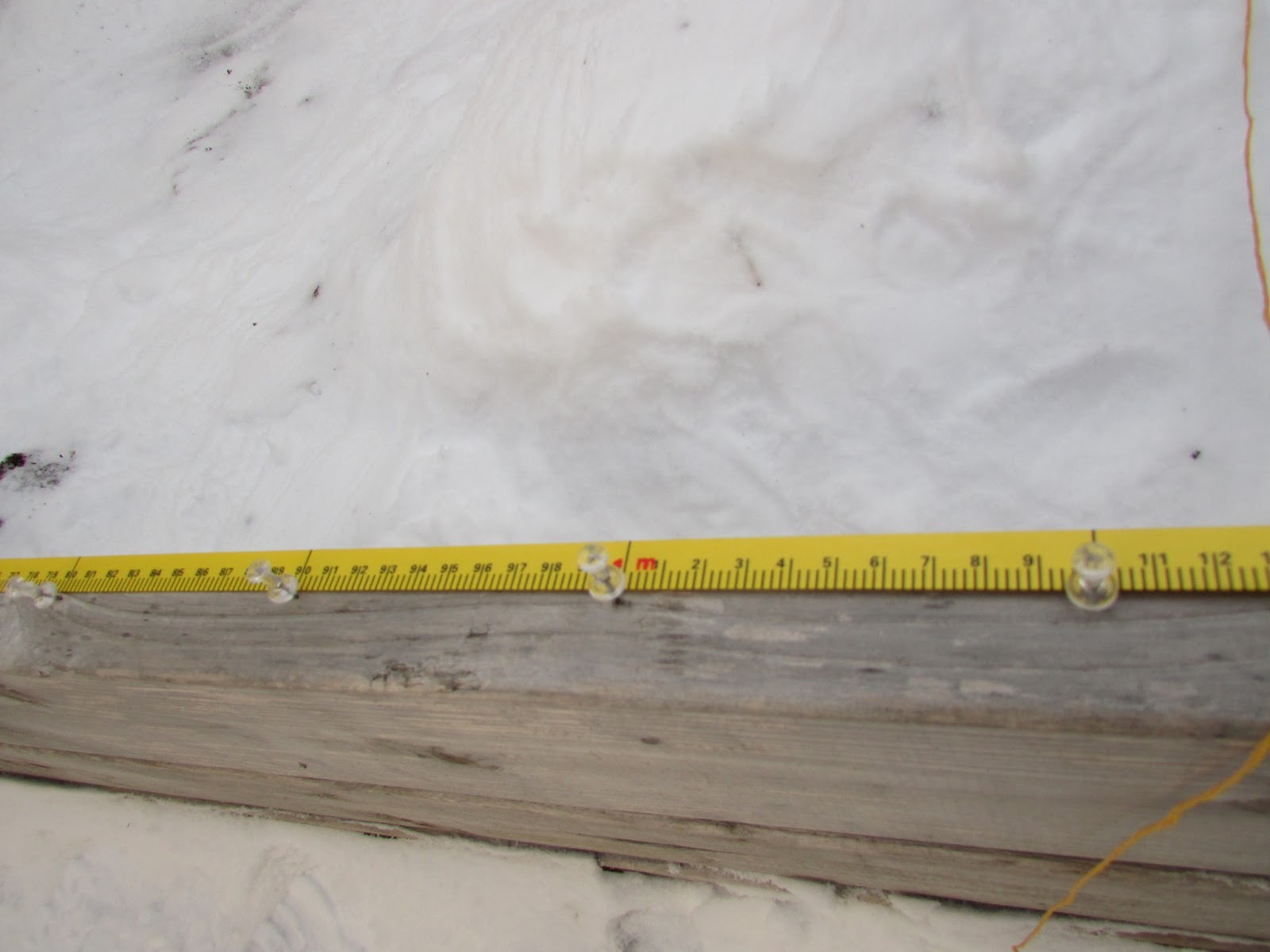Figure 13: Thumb tacks every 10 centimeters
on the x-axis.

Figure 14: Tying string to the thumb tacks.

Figure 15: Stretching string across the  box.

Figure 16: The completed coordinate system.

Once the coordinate system was complete, the team began to take measurements. To improve on our first survey, we decided to increase the amount of measurements by taking more measurements at 5 centimeter increments. The decision was made to take these finer 5 centimeter measurements on the lower part of the model and at the upper part of the model (these are the areas with greater variation in elevation). The middle of the model, which is mostly flat was still measured with 10 centimeter measurements.

The measurements were taken in much the same manner as they were in the first field activity, though we came up with a new way of measuring at the 5 centimeter intervals. It would have taken too long to put string every 5 centimeters, so the team decided to line the first string (which would have a value of 10 on the x-axis) with the 5 centimeter mark on the mobile x-axis. This ensured that an accurate 5 centimeter interval was measured exactly between two of the strings. A separate meter stick was then used to measure the negative elevation by using the value at the bottom of the mobile x-axis.  Figure 17 displays the overall measuring process, while Figures 18 and 19 display the finer details.

Figure 17: I take measurements while Laurel records.

Figure 18: Aligning the mobile x-axis with the string intervals.

Figure 19: Taking an elevation measurement.

Once all of the elevation measurements were recorded, an excel spreadsheet was created with columns for the X, Y, and Z values. Once again, 17 was added to each Z value to account for the negative measurements (-16 was the smallest integer again). After the excel spreadsheet was complete, the same procedure as earlier was used to observe the results in ArcMap and ArcScene. Figure 20 displays the new Spline Interpolation, while Figure 21 displays the terrain in ArcScene. Figure 22 displays the Spline Interpolation of the first survey for comparison.

Figure 20: Spline Interpolation of Survey 2.

Figure 21: Survey 2 displayed in ArcScene.
(the spike by the ridge is a small ice boulder)

Figure 22: Survey 1 displayed in ArcScene.

Discussion

Once again, the team encountered some problems and overcame challenges to improve on our original survey. We thought that we did fairly well with the first survey, so it was just a matter of fine-tuning our techniques. The weather was a factor once again, though it wasn't as bad as the previous activity. Laurel, Tonya, and I each worked hard to complete this second activity quickly and accurately. I think that we did quite well with the second activity, considering the weather, the new technique, and the fact that we had nearly twice as many elevation measurements in the revisit. These points make the most impact in the upper right area of the model, as can be seen when comparing Figure 21 and Figure 22. With a finer coordinate system, more data was able to be collected, giving the digital model a more realistic appearance. 

Conclusion

Our results turned out to be quite good, all things considered. We did improve on our original techniques, and increased the detail of the digital model by adding more measurement points in the upper right area of the model, covering the ridge and valley with more coordinate points. This gave our digital model a finer look, adding to the overall quality of the digital terrain model.