Enjoy!
Sunday, May 12, 2013
Final Blog: The HABL
Instead of a written description of this activity, I created a video of the HABL. Throughout the class, we have been discussing and planning a High Altitude Balloon Launch (HABL), with video imagery of the whole process. We constructed a rig, gathered the necessary materials (Weather Balloon, tracking beacon, etc.) and then waited for a morning with clear skies to finally execute the launch. The link below will take you to the video footage of the launch of this incredible activity.
Sunday, April 21, 2013
Field Activity 10: Balloon Mapping II
Introduction
This follow-up activity is very much the same as the previous activity. Using a balloon and a constructed rig, aerial photos were taken of the UW-Eau Claire campus. Once the data was collected, the images were went through and georeferenced, to be put into a mosaic and thus creating an aerial map of the campus. There was much more work put into this activity, as the last activity was just a test run of sorts.
Methodology
Much of the preparation for this activity was just as it was in the previous activity, however there are a couple noteworthy alterations. The first is that there was essentially no rig for this balloon mapping launch. It was decided that the rig contraption was not essential to the quality of the image collection (merely a very weak backup for a crash landing) so the camera was just secured to the balloon with tape and string, hanging just below the balloon. Another addition to this launch was a stabilizing wing, which was taped to the camera. This addition ensured that the camera would stay at a relatively stable position, and wouldn't be rotating constantly. One final difference was that we filled the balloon with more helium, to ensure that it would rise faster and stay more stable in the air.
After making these revisions and preparing the activity just as before, the image collection began. The balloon was released in the middle of the campus mall, and the length indicators on the string was observed to make sure the balloon reached the desired height (400 meters). Once the balloon was at the correct altitude, the class began leading the balloon around campus as the camera snapped aerial images every second (Figure 1 shows an aerial photo of our starting location). The weather was much more cooperative, with much less wind. Because of this, the class was able to collect aerial photos of the entire campus without much difficulty. We started in the middle of the campus mall, walked around the new Davies Center, walked around Phillips Hall, cut back through the mall to the footbridge, and then walked around the Haas Fine Arts Center. Once that was completed, the balloon was brought down and taken back across the footbridge, where it was once again launched to continue data collection. Because the weather was so favorable, the team lead the balloon from the footbridge to Upper Campus, collecting aerial images the entire time.
Once the data collection procedure was completed, we began to go through the images and pick out suitable images for georeferencing. Georeferencing is a procedure that positions the aerial image in the correct geospatial location by referencing a previously projected raster image (or by using Ground Control Points). For this activity, we collected several Ground Control Points, which are points that can be easily spotted on an aerial image. A team of students went around the campus with GPS units and collected the coordinates of suitable Ground Control Points (in this case, light poles were the most reliable object). We would then use these points and reference them with the corresponding objects on the aerial images so that an accurate aerial map can be created by making a mosaic. This is merely the process of forming one large image of several overlapping georeferenced images. Because the class covered such a large area, it was decided that the campus be split up into six different sections to be georeferenced by the different teams within the class (Figure 2 displays these six different sections). Each team would then submit their mosaic to create the campus aerial map.
Results
Overall, it was a very successful activity. The images that were gathered were all great, all that was required was to sort through them to find the best ones to be georeferenced. Figure 3 shows the mosaic that was created for section four (the section that my team was to georeference). Though the mosaic isn't perfect, I think that it turned out quite well considering the resources and procedures that were used to produce this result.
Discussion
I thought that this activity was a great success, especially after comparing it to the previous week's activity. The weather was perfect for what we were trying to achieve (there was no wind pushing the balloon around), and there were no other set backs to be fixed. We were all very satisfied with our results.
This follow-up activity is very much the same as the previous activity. Using a balloon and a constructed rig, aerial photos were taken of the UW-Eau Claire campus. Once the data was collected, the images were went through and georeferenced, to be put into a mosaic and thus creating an aerial map of the campus. There was much more work put into this activity, as the last activity was just a test run of sorts.
Methodology
Much of the preparation for this activity was just as it was in the previous activity, however there are a couple noteworthy alterations. The first is that there was essentially no rig for this balloon mapping launch. It was decided that the rig contraption was not essential to the quality of the image collection (merely a very weak backup for a crash landing) so the camera was just secured to the balloon with tape and string, hanging just below the balloon. Another addition to this launch was a stabilizing wing, which was taped to the camera. This addition ensured that the camera would stay at a relatively stable position, and wouldn't be rotating constantly. One final difference was that we filled the balloon with more helium, to ensure that it would rise faster and stay more stable in the air.
After making these revisions and preparing the activity just as before, the image collection began. The balloon was released in the middle of the campus mall, and the length indicators on the string was observed to make sure the balloon reached the desired height (400 meters). Once the balloon was at the correct altitude, the class began leading the balloon around campus as the camera snapped aerial images every second (Figure 1 shows an aerial photo of our starting location). The weather was much more cooperative, with much less wind. Because of this, the class was able to collect aerial photos of the entire campus without much difficulty. We started in the middle of the campus mall, walked around the new Davies Center, walked around Phillips Hall, cut back through the mall to the footbridge, and then walked around the Haas Fine Arts Center. Once that was completed, the balloon was brought down and taken back across the footbridge, where it was once again launched to continue data collection. Because the weather was so favorable, the team lead the balloon from the footbridge to Upper Campus, collecting aerial images the entire time.
 |
| Figure 1: Campus mall starting location (note the string on the right side of the image) |
 |
| Figure 2: The six different sections to be georeferenced |
Overall, it was a very successful activity. The images that were gathered were all great, all that was required was to sort through them to find the best ones to be georeferenced. Figure 3 shows the mosaic that was created for section four (the section that my team was to georeference). Though the mosaic isn't perfect, I think that it turned out quite well considering the resources and procedures that were used to produce this result.
 |
| Figure 3: The completed mosaic of section four |
I thought that this activity was a great success, especially after comparing it to the previous week's activity. The weather was perfect for what we were trying to achieve (there was no wind pushing the balloon around), and there were no other set backs to be fixed. We were all very satisfied with our results.
Sunday, April 14, 2013
Field Activity 9: Beginning Balloon Mapping
Introduction
This activity continues the work that was started in a previous activity (Activity 3). In that activity, we planned and created rigs to collect aerial photos of UW-Eau Claire's campus via balloon. Using the careful planning and constructing that was achieved during that activity (and after waiting for it to warm up a little) we were then able to finish our project.
Methods
There were several processes that had to be completed before we could actually begin the balloon mapping. First and foremost, the balloon had to be filled with helium. For this activity, we used a special weather balloon that was able to carry a payload of up to 3 lbs. While the balloon was being filled it was important to be sure that someone was always holding onto it, because it would be quite tragic if it floated away without even being used. As an extra precaution, we filled the balloon inside of the shed by Phillips Hall. Figures 1, 2, and 3 capture this process and display just how large the balloon is. Figure 3 also displays the next step, which was the securing of the balloon's opening. First, the opening is tied shut with a zip tie, then the remaining length is wrapped through a rubber ring, and then two more zip ties secure the extra length back to the original. The ring is necessary because the string will then be clipped to the balloon with a carabiner.
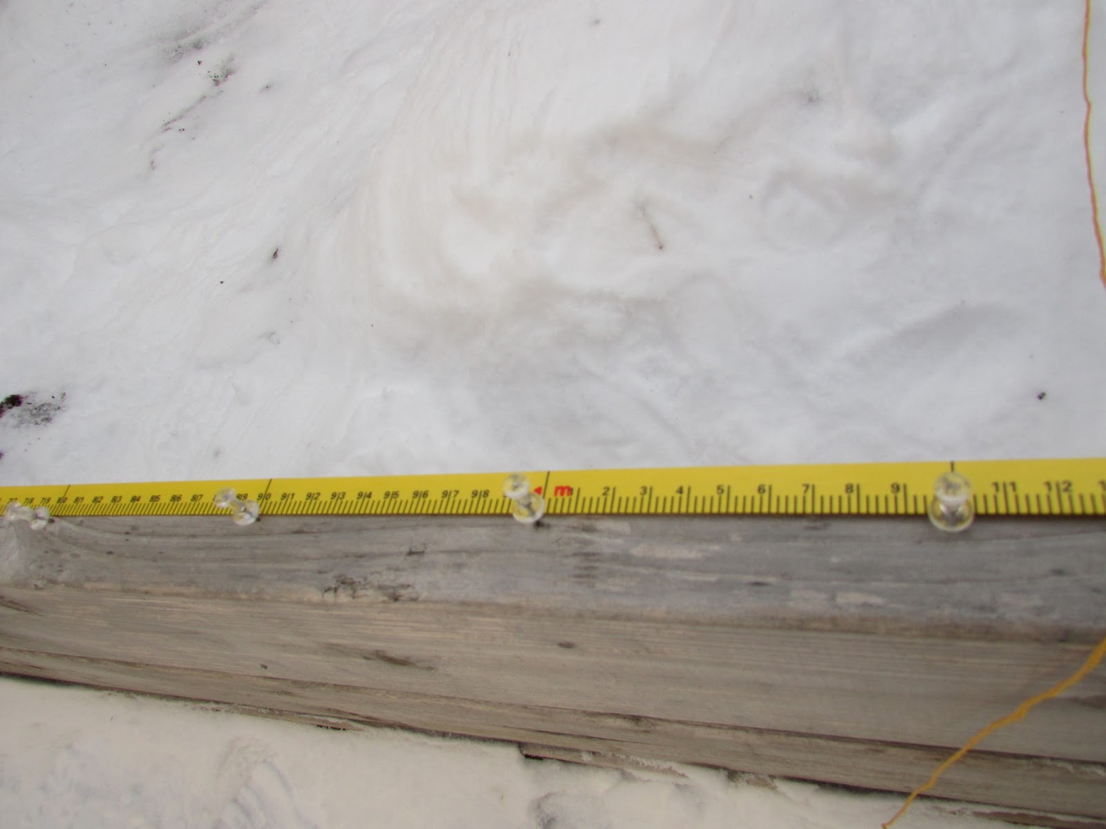
While the balloon was being filled, a team of students were required to measure out the string that would be secured to the balloon. Our target height for the balloon was 400 meters, so the team marked the string every 50 meters, and made the 400 meter mark a different color than the rest. Figure 4 shows their technique in this matter. After the string was measured, it was tied to a carabiner and then clipped on to the ring that was attached to the balloon. We then secured a GPS unit to the ring, and then tied the rig to on the string just under the balloon. After all of this preparation it was time to launch the balloon. In the middle of the campus mall the balloon was prepared for launch. The camera within the rig was set to continuous shot (so that it would take a picture every second), and then the rig was sealed. The balloon was then released, while the students holding the spool of string kept watch for the length markings (Figure 5).
This activity continues the work that was started in a previous activity (Activity 3). In that activity, we planned and created rigs to collect aerial photos of UW-Eau Claire's campus via balloon. Using the careful planning and constructing that was achieved during that activity (and after waiting for it to warm up a little) we were then able to finish our project.
Methods
There were several processes that had to be completed before we could actually begin the balloon mapping. First and foremost, the balloon had to be filled with helium. For this activity, we used a special weather balloon that was able to carry a payload of up to 3 lbs. While the balloon was being filled it was important to be sure that someone was always holding onto it, because it would be quite tragic if it floated away without even being used. As an extra precaution, we filled the balloon inside of the shed by Phillips Hall. Figures 1, 2, and 3 capture this process and display just how large the balloon is. Figure 3 also displays the next step, which was the securing of the balloon's opening. First, the opening is tied shut with a zip tie, then the remaining length is wrapped through a rubber ring, and then two more zip ties secure the extra length back to the original. The ring is necessary because the string will then be clipped to the balloon with a carabiner.
 |
| Figure 1: Preparing the balloon. |
 |
| Figure 2: Filling the balloon with helium. |
 |
| Figure 3: The balloon is filled, and the opening is secured with zip ties. A rubber loop is also attached so that the string can be clipped on with a carabiner. |
 |
| Figure 4: The string is marked in this manner every 50 meters |
 |
| Figure 5: After releasing the balloon, the string is observed to find the markings |
Once the balloon was at 400 meters, it was pulled around campus so that images were taken of most of the campus mall (Figure 6 shows the balloon and rig in flight). It was important to keep an eye on the string, and navigate away from tall objects like light poles, trees, and tall buildings. The class did this entire process twice: the first time with a standard digital camera, and a second time with a flipcam that took video footage. After the entire process, all of the data was uploaded onto a computer. We were then required to go through all of the images and select several that were perpendicular to the ground (this creates less distortion on an aerial map). Once enough suitable photos were selected, they were georeferenced and then mosaiced using either ArcMap, ERDAS Imagine, or Mapknitter.
 |
| Figure 6: The balloon, rig, and GPS unit in flight. |
Results
Because it was such a windy day, there were little suitable photos for the Mosaic process. There were several photos of Eau Claire's city horizon (Figure 7), but there was little to work with in regards to aerial mapping. However, each of us worked with what we had and a rough mosaic was created. Figure 8 displays an elementary aerial map that was created using Mapknitter.
 |
| Figure 7: With so much wind, photos such as this were quite numerous |
 |
| Figure 8: An aerial map using four aerial photos and Mapknitter. The faded background is a reference image. |
This was merely the results of our first launch, however. Our second launch was even more eventful. While we were leading the balloon across the footbridge, the string that was attached to the balloon snapped. The rig fell into the river, and the balloon floated into the distance. Luckily, the rig was a Styrofoam case and the camera was waterproof. We were able to recover both, so the data was acquired (with similar results to the previous launch).
Discussion
I thought that this activity was very exciting and a great learning experience. It was really cool to go through all of this work and then finally see the fruits of our labor. Though the wind put a damper on our plans, and the balloon dropped its payload the second time, I think that this activity was quite successful. We will be continuing this work in our next activity, hopefully with even more great results.
Sunday, April 7, 2013
Field Activity 8: Final Land Navigation
Introduction
This was the final activity in a large span of navigation activities. We began this learning experience by creating topographic maps of our study area. After this, we proceeded to learn how to navigate using the topographic map and a compass, and finally with a GPS unit. During this activity, we were to navigate to every single checkpoint on the property (15 points total), using a GPS and our maps with each checkpoint plotted. To add to the fun, each participant got an extra piece of equipment: a paintball gun. Throughout the activity we had to avoid being ambushed by other teams (or try to attack other teams), all while navigating to the checkpoints.
Study Area
For each of these activities, the class met at the University's Priory. This property is off campus and is on a 112 acre plot of forested land, perfect for navigation activities. While this location was perfect to learn these navigation techniques, it is also home to the University's Children's Center. Because we were outfitted with a paintball gun and a full face mask, we had to be careful where we navigated during the activity. Even though all the necessary authorities were notified of this activity, we did not wish to start any panic or cause any concern. Our professor stressed how important it was to avoid any areas within sight of the priory during the activity. He also advised us to stay clear of areas within sight of the highway to the north of priory, and the house to the southeast (See Figure 1 for restricted zones). With all of this in mind, as well as the massive amounts of snow on the ground, it was quite a terrain to navigate.
Methodology
Throughout this activity, we used skills that we had learned from the previous three weeks of field activities. We used navigation techniques learned from prior activities to navigate the terrain for one last time, this time trying to locate each checkpoint. For starters, we used the same map that we had made in the first navigation exersize, though it was slightly modified. This time we had to deal with restricted zones, but we also had the locations of each checkpoint on our map (Figure 2).
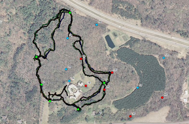
Just by looking at the map, it is easy to tell that each team would have a lot of ground to cover. After preparing for the trek (familiarizing ourselves with the paintball guns and the masks), we met up with our teams to try and come up with a strategy. Each participant used a tracklog feature on their GPS to track their navigation route once the activity was complete. Looking at Figure 2 for reference, each team started at point 1A. Our team decided to avoid traffic by going to point 6b first and then navigating around the priory to complete the course in a counter-clockwise direction. However, we were not the only team to come up with this plan. Our professor instructed us to wait 5 minutes before we could open fire, so we got to the first point with no conflict. However, after reaching that point our team lost our map so we negotiated with another team and began to work together. We then navigated by using our GPS units and our map. The basic navigation technique that we used was just looking at the lay of the land and comparing that with the topographic map to find each point. Once we were certain that we were close, we utilized the GPS units to compare more exact coordinates with the points on the map. At each checkpoint, we took a waypoint with our GPS units to mark that we had successfully navigated to that checkpoint. Figure 3 shows our teams route, as well as the waypoints at each checkpoint that we successfully navigated to. Figure 4 shows my individual tracklog, and Figure 5 shows the tracklogs of the entire class.


 Discussion
Throughout the activity, our team encountered several problems. The first and most significant problem was the loss of our map after reaching our first point. Without a map to use, we would have been quite hopeless. The map was so important because it marked where each point was, and it had a coordinate grid as well. With nothing but a GPS unit, we would have been clueless as to where to navigate. Luckily, another team agreed to help, and we continued the activity together. Not long after this, as we were navigating from point 2B to 6, we ran into another group and got into a firefight. Other than this, we ran into few other groups. Another big problem that occurred was that we were in a crunch for time towards the end of the navigation. As we navigated from point 3a to 3, we realized that there wasn't much time left. For some reason, we had trouble finding point 3 as well, so this didn't add to the situation. In the end, we decided to take a waypoint because we knew that we were quite close (this is why there is a waypoint between 3 and 2a in Figure 3). We then traveled to point 2a and then back to 1A just to find out that we still had a couple minute, and probably could have still made it to the remaining two points. I think that we relied too heavily on the map and didn't use the coordinate grid and GPS coordinates to their full potential. Also, if we had brought along the exact coordinates of the checkpoints, it would have been much easier to compare to the GPS location and we could have navigated more accurately.
Conclusion
Overall, I thought that this was a fun activity to be a part of. The addition of the paintball guns transformed the activity entirely. Not only were our navigational skills required, but we also had to stay alert for other teams that may cross our path. It added a little excitement, and I think the bruises and paint splatters that were compared afterwards can attest to that fact.
This was the final activity in a large span of navigation activities. We began this learning experience by creating topographic maps of our study area. After this, we proceeded to learn how to navigate using the topographic map and a compass, and finally with a GPS unit. During this activity, we were to navigate to every single checkpoint on the property (15 points total), using a GPS and our maps with each checkpoint plotted. To add to the fun, each participant got an extra piece of equipment: a paintball gun. Throughout the activity we had to avoid being ambushed by other teams (or try to attack other teams), all while navigating to the checkpoints.
Study Area
For each of these activities, the class met at the University's Priory. This property is off campus and is on a 112 acre plot of forested land, perfect for navigation activities. While this location was perfect to learn these navigation techniques, it is also home to the University's Children's Center. Because we were outfitted with a paintball gun and a full face mask, we had to be careful where we navigated during the activity. Even though all the necessary authorities were notified of this activity, we did not wish to start any panic or cause any concern. Our professor stressed how important it was to avoid any areas within sight of the priory during the activity. He also advised us to stay clear of areas within sight of the highway to the north of priory, and the house to the southeast (See Figure 1 for restricted zones). With all of this in mind, as well as the massive amounts of snow on the ground, it was quite a terrain to navigate.
 |
| Figure 1: Highlighted areas were the restricted zones during this activity |
Throughout this activity, we used skills that we had learned from the previous three weeks of field activities. We used navigation techniques learned from prior activities to navigate the terrain for one last time, this time trying to locate each checkpoint. For starters, we used the same map that we had made in the first navigation exersize, though it was slightly modified. This time we had to deal with restricted zones, but we also had the locations of each checkpoint on our map (Figure 2).
 |
| Figure 2: Our Starting Map |
Figure 3: Team Tracklog
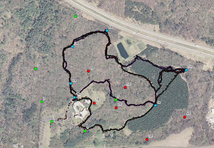
Figure 4: My Tracklog. As can be seen in the image, my GPS had some PDOP issues
because sometimes the points of the tracklog weren't quite accurate.
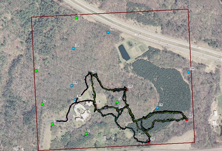
Figure 5: The tracklog of the entire class. Several different routes can be seen,
though they all seem to make the same loop.
Throughout the activity, our team encountered several problems. The first and most significant problem was the loss of our map after reaching our first point. Without a map to use, we would have been quite hopeless. The map was so important because it marked where each point was, and it had a coordinate grid as well. With nothing but a GPS unit, we would have been clueless as to where to navigate. Luckily, another team agreed to help, and we continued the activity together. Not long after this, as we were navigating from point 2B to 6, we ran into another group and got into a firefight. Other than this, we ran into few other groups. Another big problem that occurred was that we were in a crunch for time towards the end of the navigation. As we navigated from point 3a to 3, we realized that there wasn't much time left. For some reason, we had trouble finding point 3 as well, so this didn't add to the situation. In the end, we decided to take a waypoint because we knew that we were quite close (this is why there is a waypoint between 3 and 2a in Figure 3). We then traveled to point 2a and then back to 1A just to find out that we still had a couple minute, and probably could have still made it to the remaining two points. I think that we relied too heavily on the map and didn't use the coordinate grid and GPS coordinates to their full potential. Also, if we had brought along the exact coordinates of the checkpoints, it would have been much easier to compare to the GPS location and we could have navigated more accurately.
Conclusion
Overall, I thought that this was a fun activity to be a part of. The addition of the paintball guns transformed the activity entirely. Not only were our navigational skills required, but we also had to stay alert for other teams that may cross our path. It added a little excitement, and I think the bruises and paint splatters that were compared afterwards can attest to that fact.
Sunday, March 24, 2013
Activity 7: Land Navigation With GPS
Introduction
This activity was completed so that we would understand how to navigate when we do have some equipment that is a bit more up to date. Whereas in the previous activity we learned how to navigate using only the most basic technology, this activity involved using a GPS device to navigate between preset points on UW-Eau Claire's Priory property. This being said, it was a much more simple activity, because all that we had to do was navigate to the given UTM coordinates as the GPS displayed our current coordinates, as opposed to drawing bearing lines trying to stay on the set bearing.
Methodology
Much like the previous activity, we were split into teams to navigate to different points within the University's Priory property. Each team was assigned to a new course for this activity, so that we would be navigating to unfamiliar points. Zach, Laurel, and I were assigned to Course 3, and we would be doing the course in regular order instead of backwards like we had previously. Again, we were given a sheet with all the coordinates on it (Figure 1), but this time the only other materials that we needed was our GPS unit (Figure 2). Once we found our starting point, we simply had to navigate to match the coordinates on our GPS with the corresponding point coordinate.
Because the coordinate system of the area is a simple grid, it was fairly straightforward to navigate from point to point. All that our team did was determine which direction we were suppose to head by visualizing where the next point is based on the change of the coordinates. For example, going from point 1B (which had coordinates of 4957994, 617866) to point 2B (with coordinates of 4957973, 617972) required us to travel towards the E/SE direction. If you were to calculate the exact difference between the two coordinates, you would discover that point 2B is 106 meters East and 21 meters South of Point 1B. This method wasn't the most accurate, but it was the easiest to do on the run. We had no trouble finding all of the required flags (Figure 3).
Results
Throughout this exercise, our GPS units recorded tracklogs of our navigation progress. By importing these into ArcMap, we were able to visualize our navigation throughout the course and compare our results to the other team that navigated the same course as us. This was also pretty neat, because it gives us all a picture of how much land we covered as we completed the activity. The four images below display the tracklogs of our GPS units. There is an image for each course, and a single image with all of the tracklogs on it.
Discussion
This activity was quite educational and interesting. It was nice to get to explore the winter landscape once more and discover how to navigate with nothing but a GPS unit. As the figures above show, the class covered a lot of terrain, so it was quite an adventure.
This activity was completed so that we would understand how to navigate when we do have some equipment that is a bit more up to date. Whereas in the previous activity we learned how to navigate using only the most basic technology, this activity involved using a GPS device to navigate between preset points on UW-Eau Claire's Priory property. This being said, it was a much more simple activity, because all that we had to do was navigate to the given UTM coordinates as the GPS displayed our current coordinates, as opposed to drawing bearing lines trying to stay on the set bearing.
Methodology
Much like the previous activity, we were split into teams to navigate to different points within the University's Priory property. Each team was assigned to a new course for this activity, so that we would be navigating to unfamiliar points. Zach, Laurel, and I were assigned to Course 3, and we would be doing the course in regular order instead of backwards like we had previously. Again, we were given a sheet with all the coordinates on it (Figure 1), but this time the only other materials that we needed was our GPS unit (Figure 2). Once we found our starting point, we simply had to navigate to match the coordinates on our GPS with the corresponding point coordinate.
 |
| Figure 1: The coordinate sheet. Our team did course 3 (Points 1B through 6B) |
 |
| Figure 2: The GPS unit that was used for navigation |
 |
| Figure 3: Zach and I pinpoint the coordinates of a point on the course. |
Results
Throughout this exercise, our GPS units recorded tracklogs of our navigation progress. By importing these into ArcMap, we were able to visualize our navigation throughout the course and compare our results to the other team that navigated the same course as us. This was also pretty neat, because it gives us all a picture of how much land we covered as we completed the activity. The four images below display the tracklogs of our GPS units. There is an image for each course, and a single image with all of the tracklogs on it.
 |
| Figure 4: Tracklogs of the team members who completed Course 1. |
 |
| Figure 5: Tracklogs of the team members who completed Course 2. |
 |
| Figure 6: Tracklogs of the team members who completed Course 3. |
 |
| Figure 7: Tracklogs of all the students in the class. |
Discussion
This activity was quite educational and interesting. It was nice to get to explore the winter landscape once more and discover how to navigate with nothing but a GPS unit. As the figures above show, the class covered a lot of terrain, so it was quite an adventure.
Sunday, March 10, 2013
Activity 6: Traditional Land Navigation
This activity involved learning the methods of traditional land navigation (using only a topographic map and a navigation compass). It is essential to have these skills when working in the field, as we may not always have access to GPS units. We then tested our navigation skills by trekking throughout a 112 acre plot, trying to locate five previously placed flags in a certain order.
Methods
The class all met at UW-Eau Claire's Priory for this activity. With about 112 acres of forested land, it was a perfect location to do some basic land navigation. Once everyone arrived, we were given the coordinates of the different flags that we were to find (Figure 1). The coordinates of the flags were given in UTM meter units, so that we could plot them on our topographic maps from the previous activity.
 |
| Figure 1: Coordinates of the different checkpoints. |
 |
| Figure 2: Both topographic maps (one with fine contour lines, the other with an aerial background). |
 |
| Figure 3: Zach plots the checkpoints on his topographic map. |
 |
| Figure 4: Navigation map, completed with checkpoints and bearing lines. Our course started at the point to the bottom left, travelling counter clockwise. |
After we completed the plotting of our maps, we began to navigate the course. Because we were to do the course backwards, we started at point 1 and navigated to point 6, then point 5 and so on. We navigated from one point to the next by adjusting the bezel of the compass to the corresponding bearing angle, and turning our whole body to align the arrow with the case and the north-indicating needle ("putting red in the shed" as our instructor explained to us). With those two feature's aligned, the heading arrow was pointing in the correct direction. Because it wouldn't be very accurate or efficient to walk while reading a bearing (you could easily wander off course), our team worked out a great system for navigation. One person stayed put to measure the bearing, while another ran ahead. The person with the bearing would then instruct the other member on where to go to line up with the heading arrow. After everything was lined up, the team would advance to this new point. We took turns with each duty so that we all received equal experience. At first, one member of the team would measure paces so that we could calculate the distance that we've traveled, but in time we decided that it was quicker and easier to just use our navigation map as a reference. Using these methods we successfully navigated to each checkpoint with surprising accuracy.
Discussion
Our team ran into very little setbacks, and I thought that it was a quite enjoyable and beneficial experience. I've never navigated with only a compass and map, so I thought it was very interesting to finally accomplish. I'm glad that we did this activity during the winter because it would have been much more difficult to traverse the terrain with full brush. All that we had to worry about during this activity was a fresh snowfall and an advancing snowstorm.
Sunday, March 3, 2013
Activity 5: Land Nav Intro
Introduction
This short report is covering a brief intro to our upcoming land navigation activity. The point of this class' activity was to create a topographic map that would be needed to navigate the terrain at the University's Priory. We also completed a test to measure how many paces each student takes over 100 meters. Because this activity was so brief, the report will not be very extensive though a more detailed report will be completed for next week.
Methods
First, the entire class was required to test for their paces at a distance of 100 meters. To do this, a rangefinder was used to accurately measure out a 100 meter stretch. The beginning and end of this distance were then marked and it was possible to begin taking our paces. Each student walked at a steady pace while counting the number of times we make a step with our right foot.
After this was complete, the class headed in to the lab to work on our topo maps. We were encouraged to make two maps: one map with a very high detail of the topography, and one map with slightly less detailed topography but with an aerial map as a backdrop. The aerial map will be good to find a general location when navigating, while the detailed topographic map will enable us to precisely find our location. Each of these maps had a grid to help us to plot points on the map accurately.
The aerial map has contour lines at intervals of 5 meters, creating a very basic topographic map. The grid for this map is in intervals of 20 meters. The data for the 5 meter contour lines were accessed via USGS. The detailed topographic map has contour lines at intervals of 2 feet, displaying much more detailed elevation data. The grid for this map is in intervals of 25 meters (it has a larger value to decrease clutter).
Results
After finishing the pace test, I gathered results of 62.5, 61, 61.5 and 61 paces, in that order. With these results, I determined that a suitable pace for me is 61.
I am satisfied with the topographic maps that were created (Figures 1 and 2).
Discussion
This was a very simple activity, but we did encounter several problems when it came to the maps. The data for the 2 foot contour lines wasn't projected in the same coordinate system as the rest of the map data. This small setback was solved by importing the same coordinate system as the rest of the data (we decided to use NAD83 UTM Zone 15N), and viewing the entire map in that projection. We learned that it was vital to make sure that all of our data was using the correct projection, to help with the development of the map, and to ensure an accurate display. Overall, this activity was very simple yet quite informative.
This short report is covering a brief intro to our upcoming land navigation activity. The point of this class' activity was to create a topographic map that would be needed to navigate the terrain at the University's Priory. We also completed a test to measure how many paces each student takes over 100 meters. Because this activity was so brief, the report will not be very extensive though a more detailed report will be completed for next week.
Methods
First, the entire class was required to test for their paces at a distance of 100 meters. To do this, a rangefinder was used to accurately measure out a 100 meter stretch. The beginning and end of this distance were then marked and it was possible to begin taking our paces. Each student walked at a steady pace while counting the number of times we make a step with our right foot.
After this was complete, the class headed in to the lab to work on our topo maps. We were encouraged to make two maps: one map with a very high detail of the topography, and one map with slightly less detailed topography but with an aerial map as a backdrop. The aerial map will be good to find a general location when navigating, while the detailed topographic map will enable us to precisely find our location. Each of these maps had a grid to help us to plot points on the map accurately.
The aerial map has contour lines at intervals of 5 meters, creating a very basic topographic map. The grid for this map is in intervals of 20 meters. The data for the 5 meter contour lines were accessed via USGS. The detailed topographic map has contour lines at intervals of 2 feet, displaying much more detailed elevation data. The grid for this map is in intervals of 25 meters (it has a larger value to decrease clutter).
Results
After finishing the pace test, I gathered results of 62.5, 61, 61.5 and 61 paces, in that order. With these results, I determined that a suitable pace for me is 61.
I am satisfied with the topographic maps that were created (Figures 1 and 2).
 |
| Figure 1: Topographic map with contour lines at 2 foot intervals |
 |
| Figure 2: Topographic map with an aerial and contour lines at 5 meter intervals |
This was a very simple activity, but we did encounter several problems when it came to the maps. The data for the 2 foot contour lines wasn't projected in the same coordinate system as the rest of the map data. This small setback was solved by importing the same coordinate system as the rest of the data (we decided to use NAD83 UTM Zone 15N), and viewing the entire map in that projection. We learned that it was vital to make sure that all of our data was using the correct projection, to help with the development of the map, and to ensure an accurate display. Overall, this activity was very simple yet quite informative.
Sunday, February 24, 2013
Activity 4: Azimuth Survey
Introduction
The point of this activity was to learn how to use alternative methods to survey an area. Our professor emphasizes how important it is to know how to use several different surveying methods, in case high quality technology isn't at our disposal. Without high powered GPS units, a good way to survey an area is to locate a point of origin and record distance and azimuth data to survey the surrounding area. Using this method, only one GPS point is needed (or in this case, a good aerial map). It is important to understand the process first. The azimuth is a measure of the angle that you are facing (north, east, south and west). This measurement can be affected by magnetic declination, which is the difference between magnetic north and true north. As a subject's location gets farther from the line where true north is constant, declination increases. To make up for this, degrees must be added or subtracted from the azimuth, depending on how much declination there is, and whether it is positive or negative. Luckily here in Eau Claire, the magnetic declination is merely 0 degrees 58 minutes West, which is too minimal to account for in our survey.
Methods
This was a fairly straight forward activity. All that was required was either a sonic range finder and a compass, or a laser range finder that also calculates azimuth. During the class, we each familiarized ourselves with the new gear, as we haven't used it before. To test everything out, we simply went behind Phillips Hall and recorded data using a distinctive tree as an origin point. Using the laser range finder, I recorded the distance and azimuth of two art structures, an emergency phone, and several trees. Once everyone had done the same, we entered the data into ArcGIS by creating an Excel spreadsheet and used the Bearing Distance to Line tool to create a feature from the recorded data. Before this, however, it was necessary to locate the origin tree and find out the latitude and longitude values of its position by using an aerial map. The completed feature was quite accurate, with only minor variance from accidentally moving (inconsistent origin).
Now that we had familiarized ourselves with the gear and the computer lab work, it was time to conduct our own survey on the UW-EC campus. Laurel and I decided to survey the stone benches on the new campus mall. First, I checked the aerial map to look for suitable locations to use as an origin point. We chose to use the library entrance as the origin because it is a slightly elevated platform and would have a good view of most of the campus mall. Midway through the survey, we had to select a second origin because some of the benches weren't in view. For this second origin point, we chose the doorway to Schofield Hall. We had to make sure we would be able to find it in an aerial map, and the doorway was perfect.
Laurel and I had a good process to record the azimuth and distance data. I used the laser range finder to calculate the distance and azimuth while she recorded the data in a notepad, collecting 41 points total. The field work was surprisingly quick with the laser range finder. After the data was collected, Laurel made an Excel spreadsheet of the data, which was then entered into ArcGIS like we previously did. Then, using the Bearing Distance to Line tool, we once again created features of the data. We had to make special note of which points were collected at which origin, since we had more than one.
Results
Once again, the data was surprisingly accurate. Figure 1 displays our work. There does appear to be a lot of open space between the two origins, which could be from slightly skewed data or missed benches completely (it had just snowed before we took the survey).
Discussion
I thought that the survey went quite well, and it was a quick and easy process as well. This activity was quite fun and I think that the methods we learned will come in useful later in my career. It would have been nice to be able to check our results and see how accurate our survey was, but our campus was too new to have a recent aerial photo. All in all the entire activity went well.
The point of this activity was to learn how to use alternative methods to survey an area. Our professor emphasizes how important it is to know how to use several different surveying methods, in case high quality technology isn't at our disposal. Without high powered GPS units, a good way to survey an area is to locate a point of origin and record distance and azimuth data to survey the surrounding area. Using this method, only one GPS point is needed (or in this case, a good aerial map). It is important to understand the process first. The azimuth is a measure of the angle that you are facing (north, east, south and west). This measurement can be affected by magnetic declination, which is the difference between magnetic north and true north. As a subject's location gets farther from the line where true north is constant, declination increases. To make up for this, degrees must be added or subtracted from the azimuth, depending on how much declination there is, and whether it is positive or negative. Luckily here in Eau Claire, the magnetic declination is merely 0 degrees 58 minutes West, which is too minimal to account for in our survey.
Methods
This was a fairly straight forward activity. All that was required was either a sonic range finder and a compass, or a laser range finder that also calculates azimuth. During the class, we each familiarized ourselves with the new gear, as we haven't used it before. To test everything out, we simply went behind Phillips Hall and recorded data using a distinctive tree as an origin point. Using the laser range finder, I recorded the distance and azimuth of two art structures, an emergency phone, and several trees. Once everyone had done the same, we entered the data into ArcGIS by creating an Excel spreadsheet and used the Bearing Distance to Line tool to create a feature from the recorded data. Before this, however, it was necessary to locate the origin tree and find out the latitude and longitude values of its position by using an aerial map. The completed feature was quite accurate, with only minor variance from accidentally moving (inconsistent origin).
Now that we had familiarized ourselves with the gear and the computer lab work, it was time to conduct our own survey on the UW-EC campus. Laurel and I decided to survey the stone benches on the new campus mall. First, I checked the aerial map to look for suitable locations to use as an origin point. We chose to use the library entrance as the origin because it is a slightly elevated platform and would have a good view of most of the campus mall. Midway through the survey, we had to select a second origin because some of the benches weren't in view. For this second origin point, we chose the doorway to Schofield Hall. We had to make sure we would be able to find it in an aerial map, and the doorway was perfect.
Laurel and I had a good process to record the azimuth and distance data. I used the laser range finder to calculate the distance and azimuth while she recorded the data in a notepad, collecting 41 points total. The field work was surprisingly quick with the laser range finder. After the data was collected, Laurel made an Excel spreadsheet of the data, which was then entered into ArcGIS like we previously did. Then, using the Bearing Distance to Line tool, we once again created features of the data. We had to make special note of which points were collected at which origin, since we had more than one.
Results
Once again, the data was surprisingly accurate. Figure 1 displays our work. There does appear to be a lot of open space between the two origins, which could be from slightly skewed data or missed benches completely (it had just snowed before we took the survey).
 |
| Figure 1: The red lines display the data collected from the library entrance and the blue lines display the data collected from the Schofield Hall doorway. Unfortunately there is no aerial photo to compare the results to. |
Discussion
I thought that the survey went quite well, and it was a quick and easy process as well. This activity was quite fun and I think that the methods we learned will come in useful later in my career. It would have been nice to be able to check our results and see how accurate our survey was, but our campus was too new to have a recent aerial photo. All in all the entire activity went well.
Sunday, February 17, 2013
Activity 3: Equipment Construction & Testing
Introduction
This activity was a prep session for the activity that we will be doing next week. The class plans to use a balloon rig to take aerial photos of the campus. We will also be conducting a high altitude balloon launch (HABL), with a camera rigged to it. During this activity, we simply needed to construct the rigs for both, and test all the equipment to ensure that the launching of the balloons is smooth and successful. The class was not split in to groups for this activity so it was somewhat unorganized, but I mostly helped with the construction of one of the balloon mapping rigs.
Methods
As said before, this activity was a prep for the next. There were several different things that needed to be prepared and tested during this activity. The list consisted of construction of a mapping rig, construction of the HABL rig, parachute testing, payload weight, testing the continuous shot on the cameras, and testing of the tracking device. I mostly helped out with the construction of one of the mapping rigs (two designs were created) so this methodology will consist of the process of the mapping rigs construction.
Our design for the mapping rig included the use of a one gallon Rain X bottle, a camera, string, tape, and scissors. The main idea was to mount a downward facing camera inside the Rain X bottle with the bottom removed. The first step of this process was of course removing the bottom of the Rain X bottle. It was necessary to leave enough length for the camera to hang, and have a length below the camera so that when the rig lands, the camera isn't damaged.
Once we finished the rig's casing, we had to come up with a design to hang the camera inside of it. Our design calls for 1.5 meters of string that is tied into a loop. Two ends of this loop are then wrapped around the camera, securing the string to the camera with tape. The length of the string that isn't secured to the camera is then pulled through the bottom of the casing and out the nozzle on the top of the bottle. The string would then be attached to the balloon. In order to keep the camera hanging freely within the case, and not pulled to the top by the balloon, another length of string was attached to the camera, pulled out the top of the casing, and then tied securely to notch at the bottom of the plastic bottle casing. Figures 2 through 5 show the camera rigging in detail.
The final touch to the rig are the stabilizing wings on the handle of the plastic bottle. These were made by cutting a six inch section off of the side of a 2 liter pop bottle. The wings were then securely taped to the rig's casing. These wings are necessary to stabilize the rig, and reduce spin from wind when the rig is in the air. With less spin, we would be able to collect more consistent images, and make it easier to mosaic when we make the aerial map in our next activity. Figure 6 shows this final step.
Discussion
This activity was a prep session for the activity that we will be doing next week. The class plans to use a balloon rig to take aerial photos of the campus. We will also be conducting a high altitude balloon launch (HABL), with a camera rigged to it. During this activity, we simply needed to construct the rigs for both, and test all the equipment to ensure that the launching of the balloons is smooth and successful. The class was not split in to groups for this activity so it was somewhat unorganized, but I mostly helped with the construction of one of the balloon mapping rigs.
Methods
As said before, this activity was a prep for the next. There were several different things that needed to be prepared and tested during this activity. The list consisted of construction of a mapping rig, construction of the HABL rig, parachute testing, payload weight, testing the continuous shot on the cameras, and testing of the tracking device. I mostly helped out with the construction of one of the mapping rigs (two designs were created) so this methodology will consist of the process of the mapping rigs construction.
 |
| Figure 1: The rigs plastic bottle casing. |
 |
| Figure 2: Rigging the camera. |
 |
| Figure 3: A look at the camera's face. |
 |
| Figure 4: The camera as it hangs. |
 |
| Figure 5: The camera within the casing (note the additional rigging on the bottom of the casing). |
 |
| Figure 6: The rig's casing with attached wings. |
I thought that this activity went pretty well, even though it was a bit unorganized. The rig that we worked on did turn out well, but it seemed to me like the work wasn't evenly spread out. It would've helped if we had been divided into groups again, and assigned what to work on so that each person had something to work on.
Results
The overall results of this activity were quite well. The class completed everything on the list that needed to be prepared and tested, including two different balloon mapping rigs, a HABL rig, parachute testing, camera testing, and equipment weighing. We now have nearly everything ready to begin the next activity (everything except the balloon prep, which would of course need to wait until the launch day anyway). Figures 7 through 10 show projects that other students worked on and completed with this activity.
 |
| Figure 7: Completed balloon mapping rig #1. |
 |
| Figure 8: Completed balloon mapping rig #2. |
 |
| Figure 9: Parachute testing |
 |
| Figure 10: HABL rig |
Sunday, February 10, 2013
Field Activity 2: Survey Revisit
This activity was conducted to experience a vital procedure in field work: a revisit of the first Field Activity. During this activity, we looked for ways to improve on the first activity by trying to find flawed areas or coming up with new procedures that enable us to report more precise results. Where the first activity was learning how to work on the field with minimal equipment, this activity is learning how to improve our procedures by observing our previous results.
Methods
First, the team analyzed the data that was collected from Field Activity 1. This was done by importing the X,Y,Z excel spreadsheet into ArcMap and using several different Raster Interpolation tools to display the elevation data, each with varying results. The different techniques that were used included IDW, Kriging, Natural Neighbor, and Spline interpolations. These interpolations were then displayed in 3D using ArcScene. Figures 1 through 8 display the results of each of these procedures.
 |
| Figure 1: IDW Interpolation - Uses an inverse distance weighted technique to interpolate the data. |
 |
| Figure 2: IDW technique in ArcScene. |
 |
| Figure 3: Kriging Interpolation - uses a Kriging procedure to interpolate the data. |
 |
| Figure 4: Kriging technique in ArcScene. |
 |
| Figure 5: Natural Neighbor Interpolation - Uses a balance of data between neighboring points to interpolate the raster. |
 |
| Figure 6: Natural Neighbor Interpolation in ArcScene. |
 |
| Figure 7: Spline Interpolation - Uses a two-dimensional minimum curvature spline technique to interpolate the raster. |
 |
| Figure 8: Spline Interpolation in ArcScene. |
The first area that was looked to improve on is the gear that is worn in the field. Learning from the past activity (the team had to work in extremely cold weather, with temperatures hovering around 0 degrees Fahrenheit) was extremely important here. Each team member was bundled up in their warmest clothes, as the temperature was still going to be quite cold (around 25 degrees Fahrenheit). Figure 9 is a fine example of this preparation process. After preparing for the cold weather, the necessary supplies were gathered and the team was ready to go. For this survey, the supplies used were meter sticks, measuring tape, string, and thumb tacks.
 |
| Figure 9: Preparing for the cold weather. |
 |
| Figure 10: Tonya and I observing the remains of the terrain model. |
 |
| Figure 11: Laurel and I packing the model down to its original form. |
With the terrain model restored, the team began to construct the coordinate system with a new and improved technique. It was decided that we should keep the measuring tape along both sides of the y-axis (Figure 12), but we decided to improve the original design by measuring out the x-axis at 10 centimeter intervals and pulling string across the box on each of these points (Figures 13 through 15?). This process would help to make the measuring process quicker and more precise. Figure 16 displays the completed coordinate system.
 |
| Figure 12: Tonya applying the measuring tape to the y-axis. |
 |
| Figure 13: Thumb tacks every 10 centimeters on the x-axis. |
 |
| Figure 14: Tying string to the thumb tacks. |
 |
| Figure 15: Stretching string across the box. |
 |
| Figure 16: The completed coordinate system. |
Once the coordinate system was complete, the team began to take measurements. To improve on our first survey, we decided to increase the amount of measurements by taking more measurements at 5 centimeter increments. The decision was made to take these finer 5 centimeter measurements on the lower part of the model and at the upper part of the model (these are the areas with greater variation in elevation). The middle of the model, which is mostly flat was still measured with 10 centimeter measurements.
The measurements were taken in much the same manner as they were in the first field activity, though we came up with a new way of measuring at the 5 centimeter intervals. It would have taken too long to put string every 5 centimeters, so the team decided to line the first string (which would have a value of 10 on the x-axis) with the 5 centimeter mark on the mobile x-axis. This ensured that an accurate 5 centimeter interval was measured exactly between two of the strings. A separate meter stick was then used to measure the negative elevation by using the value at the bottom of the mobile x-axis. Figure 17 displays the overall measuring process, while Figures 18 and 19 display the finer details.
 |
| Figure 17: I take measurements while Laurel records. |
 |
| Figure 18: Aligning the mobile x-axis with the string intervals. |
 |
| Figure 19: Taking an elevation measurement. |
Once all of the elevation measurements were recorded, an excel spreadsheet was created with columns for the X, Y, and Z values. Once again, 17 was added to each Z value to account for the negative measurements (-16 was the smallest integer again). After the excel spreadsheet was complete, the same procedure as earlier was used to observe the results in ArcMap and ArcScene. Figure 20 displays the new Spline Interpolation, while Figure 21 displays the terrain in ArcScene. Figure 22 displays the Spline Interpolation of the first survey for comparison.
 |
| Figure 20: Spline Interpolation of Survey 2. |
 |
| Figure 21: Survey 2 displayed in ArcScene. (the spike by the ridge is a small ice boulder) |
|
| Figure 22: Survey 1 displayed in ArcScene. |
Discussion
Once again, the team encountered some problems and overcame challenges to improve on our original survey. We thought that we did fairly well with the first survey, so it was just a matter of fine-tuning our techniques. The weather was a factor once again, though it wasn't as bad as the previous activity. Laurel, Tonya, and I each worked hard to complete this second activity quickly and accurately. I think that we did quite well with the second activity, considering the weather, the new technique, and the fact that we had nearly twice as many elevation measurements in the revisit. These points make the most impact in the upper right area of the model, as can be seen when comparing Figure 21 and Figure 22. With a finer coordinate system, more data was able to be collected, giving the digital model a more realistic appearance.
Conclusion
Our results turned out to be quite good, all things considered. We did improve on our original techniques, and increased the detail of the digital model by adding more measurement points in the upper right area of the model, covering the ridge and valley with more coordinate points. This gave our digital model a finer look, adding to the overall quality of the digital terrain model.
Subscribe to:
Posts (Atom)