Activity 7: Land Navigation With GPS

Introduction
This activity was completed so that we would understand how to navigate when we do have some equipment that is a bit more up to date. Whereas in the previous activity we learned how to navigate using only the most basic technology, this activity involved using a GPS device to navigate between preset points on UW-Eau Claire's Priory property. This being said, it was a much more simple activity, because all that we had to do was navigate to the given UTM coordinates as the GPS displayed our current coordinates, as opposed to drawing bearing lines trying to stay on the set bearing.

Methodology
Much like the previous activity, we were split into teams to navigate to different points within the University's Priory property. Each team was assigned to a new course for this activity, so that we would be navigating to unfamiliar points. Zach, Laurel, and I were assigned to Course 3, and we would be doing the course in regular order instead of backwards like we had previously. Again, we were given a sheet with all the coordinates on it (Figure 1), but this time the only other materials that we needed was our GPS unit (Figure 2). Once we found our starting point, we simply had to navigate to match the coordinates on our GPS with the corresponding point coordinate.

Figure 1: The coordinate sheet. Our team did course 3 (Points 1B through 6B)

Figure 2: The GPS unit that was used for navigation

Because the coordinate system of the area is a simple grid, it was fairly straightforward to navigate from point to point. All that our team did was determine which direction we were suppose to head by visualizing where the next point is based on the change of the coordinates. For example, going from point 1B (which had coordinates of 4957994, 617866) to point 2B (with coordinates of 4957973, 617972) required us to travel towards the E/SE direction. If you were to calculate the exact difference between the two coordinates, you would discover that point 2B is 106 meters East and 21 meters South of Point 1B. This method wasn't the most accurate, but it was the easiest to do on the run. We had no trouble finding all of the required flags (Figure 3).

Figure 3: Zach and I pinpoint the coordinates of a point on the course.

Results
Throughout this exercise, our GPS units recorded tracklogs of our navigation progress. By importing these into ArcMap, we were able to visualize our navigation throughout the course and compare our results to the other team that navigated the same course as us. This was also pretty neat, because it gives us all a picture of how much land we covered as we completed the activity. The four images below display the tracklogs of our GPS units. There is an image for each course, and a single image with all of the tracklogs on it.

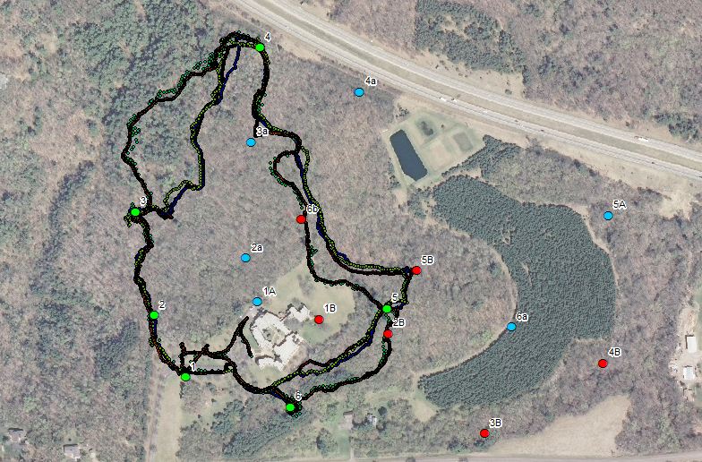
Figure 4: Tracklogs of the team members who completed Course 1.

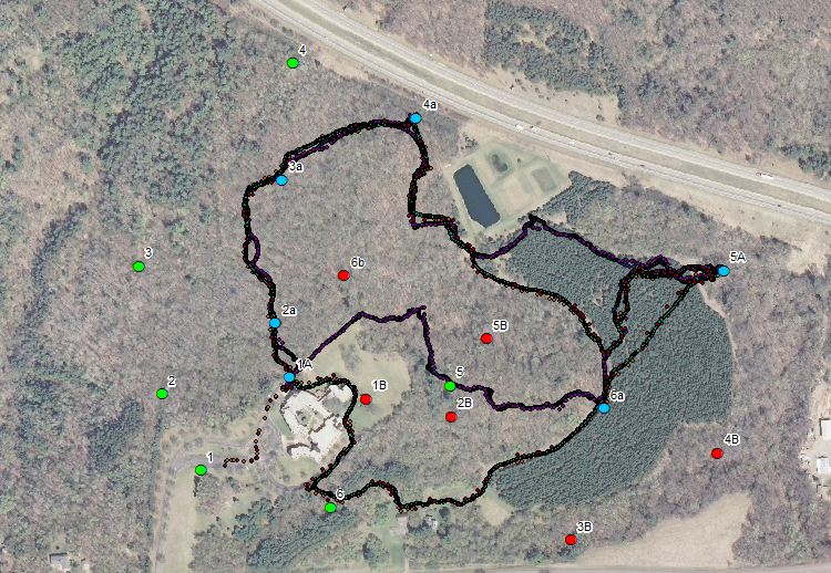
Figure 5: Tracklogs of the team members who completed Course 2.

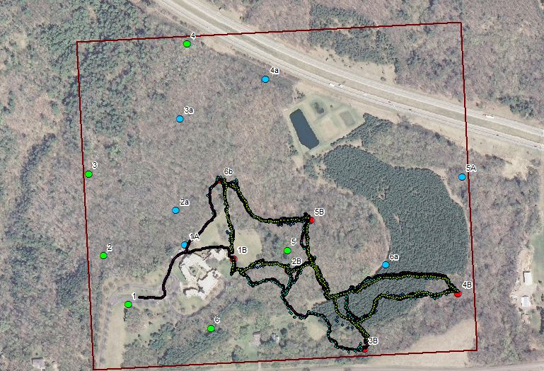
Figure 6: Tracklogs of the team members who completed Course 3.

Figure 7: Tracklogs of all the students in the class.

Discussion
This activity was quite educational and interesting. It was nice to get to explore the winter landscape once more and discover how to navigate with nothing but a GPS unit. As the figures above show, the class covered a lot of terrain, so it was quite an adventure.

Activity 6: Traditional Land Navigation

Introduction
This activity involved learning the methods of traditional land navigation (using only a topographic map and a navigation compass). It is essential to have these skills when working in the field, as we may not always have access to GPS units. We then tested our navigation skills by trekking throughout a 112 acre plot, trying to locate five previously placed flags in a certain order.

Methods
The class all met at UW-Eau Claire's Priory for this activity. With about 112 acres of forested land, it was a perfect location to do some basic land navigation. Once everyone arrived, we were given the coordinates of the different flags that we were to find (Figure 1). The coordinates of the flags were given in UTM meter units, so that we could plot them on our topographic maps from the previous activity.

Figure 1: Coordinates of the different checkpoints.

There were three different courses, each with five checkpoints that needed to be located. Because there were six different groups, two groups shared one course (however one of these teams had to do the course backwards). Each of the checkpoints had a paper punch so that we had proof of arriving at the destination. Zach, Laurel, and I were selected to do course number two backwards. With these coordinates, we then began to plot the points on our previously made topographic maps (Figures 2 and 3). To do this, we simply located the checkpoint on the map by plotting the data in the UTM_Y and UTM_X columns for our five points. Because some of these points were quite a distance from each other, we traced a line from point to point so that we could measure the proper bearing angle with more accuracy. Figure 4 displays a completed map with plotted points and bearing lines.

Figure 2: Both topographic maps (one with fine contour
lines, the other with an aerial background).

Figure 3: Zach plots the checkpoints on his topographic
map.

Figure 4: Navigation map, completed with checkpoints and bearing lines.
Our course started at the point to the bottom left, travelling counter clockwise.

Once we each completed our navigation maps, we used navigation compasses to measure for the bearing angle from each point to the next. With the bearing lines traced onto the map, this was a simple procedure. To find the bearing angle, we just lined up the compass with the bearing line (making sure the heading arrow was pointing the right way), and then adjusted the bezel of the compass so that the arrow within its casing was pointing to the map's true north. The bearing angle would then be the value that is indicated by the heading arrow on the base of the compass. We measured the bearing for each angle and recorded the values on the map so that we could use them quickly in the field. Lastly, we measured the distances between the points on the course, using the map's scale bar and the ruler on the side of the compass. The distances were recorded so that we could pace while we navigate and have a basic idea of how much further we had to go. 

After we completed the plotting of our maps, we began to navigate the course. Because we were to do the course backwards, we started at point 1 and navigated to point 6, then point 5 and so on. We navigated from one point to the next by adjusting the bezel of the compass to the corresponding bearing angle, and turning our whole body to align the arrow with the case and the north-indicating needle ("putting red in the shed" as our instructor explained to us). With those two feature's aligned, the heading arrow was pointing in the correct direction. Because it wouldn't be very accurate or efficient to walk while reading a bearing (you could easily wander off course), our team worked out a great system for navigation. One person stayed put to measure the bearing, while another ran ahead. The person with the bearing would then instruct the other member on where to go to line up with the heading arrow. After everything was lined up, the team would advance to this new point. We took turns with each duty so that we all received equal experience. At first, one member of the team would measure paces so that we could calculate the distance that we've traveled, but in time we decided that it was quicker and easier to just use our navigation map as a reference. Using these methods we successfully navigated to each checkpoint with surprising accuracy.

Discussion

Our team ran into very little setbacks, and I thought that it was a quite enjoyable and beneficial experience. I've never navigated with only a compass and map, so I thought it was very interesting to finally accomplish. I'm glad that we did this activity during the winter because it would have been much more difficult to traverse the terrain with full brush. All that we had to worry about during this activity was a fresh snowfall and an advancing snowstorm.

Activity 5: Land Nav Intro

Introduction
This short report is covering a brief intro to our upcoming land navigation activity. The point of this class' activity was to create a topographic map that would be needed to navigate the terrain at the University's Priory. We also completed a test to measure how many paces each student takes over 100 meters. Because this activity was so brief, the report will not be very extensive though a more detailed report will be completed for next week.

Methods
First, the entire class was required to test for their paces at a distance of 100 meters. To do this, a rangefinder was used to accurately measure out a 100 meter stretch. The beginning and end of this distance were then marked and it was possible to begin taking our paces. Each student walked at a steady pace while counting the number of times we make a step with our right foot.

After this was complete, the class headed in to the lab to work on our topo maps. We were encouraged to make two maps: one map with a very high detail of the topography, and one map with slightly less detailed topography but with an aerial map as a backdrop. The aerial map will be good to find a general location when navigating, while the detailed topographic map will enable us to precisely find our location. Each of these maps had a grid to help us to plot points on the map accurately.

The aerial map has contour lines at intervals of 5 meters, creating a very basic topographic map. The grid for this map is in intervals of 20 meters. The data for the 5 meter contour lines were accessed via USGS. The detailed topographic map has contour lines at intervals of 2 feet, displaying much more detailed elevation data. The grid for this map is in intervals of 25 meters (it has a larger value to decrease clutter).

Results
After finishing the pace test, I gathered results of 62.5, 61, 61.5 and 61 paces, in that order. With these results, I determined that a suitable pace for me is 61.

I am satisfied with the topographic maps that were created (Figures 1 and 2).

Figure 1: Topographic map with contour lines at 2 foot intervals

Figure 2: Topographic map with an aerial and contour lines at 5 meter intervals

Discussion
This was a very simple activity, but we did encounter several problems when it came to the maps. The data for the 2 foot contour lines wasn't projected in the same coordinate system as the rest of the map data. This small setback was solved by importing the same coordinate system as the rest of the data (we decided to use NAD83 UTM Zone 15N), and viewing the entire map in that projection. We learned that it was vital to make sure that all of our data was using the correct projection, to help with the development of the map, and to ensure an accurate display. Overall, this activity was very simple yet quite informative.